Hedonic imputation with one regression, not two

Hedonic imputation is a standard method to compare prices over time when the composition of products also changes. In all cases I’ve seen, the method is implemented by using the fitted values from two regression models. I show how it can be done with one regression.

Comparing housing prices over time is difficult because of all the heterogeneity in housing that can both affect prices and vary over time. The typical solution to this problem is to use a hedonic price index that attempts to model the relationship between housing characteristics and price, and uses this to control the change in these characteristics over time.

Although there are several approaches to building a hedonic price index, the double imputation approach is usually seen as the best. Every presentation of this method that I have seen calculates the index by fitting two regression models and combining the fitted values from these models in a geometric index (e.g., Aizcorbe 2014; ILO et al. 2013; IMF 2020). What I want to show here is that the double imputation index can be recovered from the coefficient in a linear regression. This makes it simpler to calculate the index and provides an easy strategy to estimate conventional standard errors.

Turning two regressions into one

The hedonic imputation model starts with two linear models, one for transactions in period 0,

\[ \log(p_{i0}) = \alpha_{0} + x_{i0} \beta_{0} + u_{i0}, \tag{1}\]

and one for transactions in period 1,

\[ \log(p_{i1}) = \alpha_{1} + x_{i1} \beta_{1} + e_{i1}, \tag{2}\]

where \(x_{it}\) is a vector of characteristics that confound a change in price over time with a change in the composition of housing.

The Laspeyres hedonic imputation index, \(I\), compares the predicted prices from Equation 2 against those from Equation 1 over the distribution of characteristics in period 0

\[ \log(I) = \alpha_{1} - \alpha_{0} + \bar{x}_{0} (\beta_{1} - \beta_{0}), \tag{3}\]

where \(\bar{x}_{0}\) is the vector of average period 0 characteristics. This is equation 5.19 in ILO et al. (2013).

Equation 1 and Equation 2 can be nested to get a single linear model. Subtracting \(\bar{x}_{0}\) from the interaction term then gives Equation 3 as a coefficient on a time dummy variable

\[\begin{align} \log(p_{it}) &= \alpha_{0} + x_{it} \beta_{0} + t (\alpha_{1} - \alpha_{0} + x_{it} (\beta_{1} - \beta_{0})) + u_{it} + t(e_{it} - u_{it})\\ &= \alpha_{0} + t \log(I) + x_{it} \beta_{0} + t (x_{it} - \bar{x}_{0}) (\beta_{1} - \beta_{0}) + \varepsilon_{it}, \end{align}\]

where \(\varepsilon_{it} = u_{it} + t(e_{it} - u_{it})\). The Paasche hedonic imputation index follows along the same lines, replacing \(\bar{x}_{0}\) with \(\bar{x}_{1}\). The Fisher hedonic imputation index combines these two, which is the same as replacing \(\bar{x}_{0}\) with \(\bar{x}_{0} / 2 + \bar{x}_{1} / 2\). Note that this reduces to the classic time-dummy hedonic index when \(\beta_{1} = \beta_{0}\).¹

An example

Let’s go through an example to see this in action. As the goal is just to give an example, I’ll make up some typical-looking transaction data for property sales with a few characteristics over two periods.

set.seed(15243)

sales <- data.frame(
  period = rep(0:1, c(120, 180)),
  price = rlnorm(300),
  area = runif(300, 800, 2500),
  age = sample(1:80, 300, replace = TRUE),
  amenity_score = runif(300)
)

head(sales)

  period     price      area age amenity_score
1      0 1.8931980 2415.7592  70    0.01447159
2      0 0.9737266 2244.8349   5    0.59602963
3      0 0.9860096 1937.4438  80    0.39965375
4      0 1.4830738  989.7379  66    0.16038727
5      0 0.3651522 2324.3656  50    0.82509594
6      0 0.7955844 1930.3795  12    0.38836734

We’ll work with the following basic model relating price with characteristics in each period

\[ \log(\text{price}_{it}) = \alpha_{t} + \beta_{1t}\text{age}_{it} + \beta_{2t}\text{area}_{it} + \beta_{i3}\text{area}_{it}^2 + \beta_{i4}\text{neighbourhoodscore}_{it} + \varepsilon_{it}. \]

The two-regression approach for making the Laspeyres-imputation index fits two separate models for each time period and compares the average ratio of predicted prices over the distribution of housing characteristics for sales in period 0.

sales2 <- split(sales, ~period)

mdl1 <- lm(log(price) ~ age + area + I(area^2) + amenity_score, sales2[[1]])

mdl2 <- lm(log(price) ~ age + area + I(area^2) + amenity_score, sales2[[2]])

laspeyres <- exp(mean(predict(mdl2, sales2[[1]]) - predict(mdl1, sales2[[1]])))

laspeyres

[1] 0.9367763

The Paasche-imputation index does the same thing, just over the distribution of characteristics for sales in period 1, and the Fisher-imputation index combines the Laspeyres and Paasche indexes.

paasche <- exp(mean(predict(mdl2, sales2[[2]]) - predict(mdl1, sales2[[2]])))

paasche

[1] 0.9376688

fisher <- sqrt(laspeyres * paasche)

fisher

[1] 0.9372224

To make these indexes with one regression we need to remove the appropriate mean from the characteristics variables and interact them with the time dummy in the linear model. In each case the coefficient on the time dummy variable gives the same index as using two regressions. For simplicity, I’ll just show the case of the Fisher index.

dm <- function(x) {
  m0 <- mean(x[eval(substitute(period == 0), parent.frame())])
  m1 <- mean(x[eval(substitute(period == 1), parent.frame())])
  x - mean(c(m0, m1))
}

mdl_fisher <- lm(
  log(price) ~ period +
    age +
    area +
    I(area^2) +
    amenity_score +
    period:(dm(age) + dm(area) + dm(area^2) + dm(amenity_score)),
  sales
)

all.equal(exp(coef(mdl_fisher)["period"]), fisher, check.attributes = FALSE)

[1] TRUE

Representing the Fisher index as the coefficient in a linear model also makes it easy to get the (delta method) standard error for the index. ²

exp(coef(mdl_fisher)["period"]) * sqrt(sandwich::vcovHC(mdl_fisher)[2, 2])

   period 
0.1009944 

Adding weights to both the regression model and the index-number formulas is a simple extension. Continuing with the above example, suppose we want to weight by house price so that more expensive houses received a larger weight.

mdl1 <- lm(
  log(price) ~ age + area + I(area^2) + amenity_score,
  sales2[[1]],
  weights = price
)

mdl2 <- lm(
  log(price) ~ age + area + I(area^2) + amenity_score,
  sales2[[2]],
  weights = price
)

laspeyres <- exp(
  weighted.mean(
    predict(mdl2, sales2[[1]]) - predict(mdl1, sales2[[1]]),
    sales2[[1]]$price
  )
)

paasche <- exp(
  weighted.mean(
    predict(mdl2, sales2[[2]]) - predict(mdl1, sales2[[2]]),
    sales2[[2]]$price
  )
)

fisher <- sqrt(laspeyres * paasche)

Making the Fisher index with one regression just requires removing the weighted mean from the characteristics variables in the interaction term.

dm <- function(x) {
  m0 <- eval(
    substitute(weighted.mean(x[period == 0], price[period == 0])),
    parent.frame()
  )
  m1 <- eval(
    substitute(weighted.mean(x[period == 1], price[period == 1])),
    parent.frame()
  )
  x - mean(c(m0, m1))
}

mdl_fisher <- lm(
  log(price) ~ period +
    age +
    area +
    I(area^2) +
    amenity_score +
    period:(dm(age) + dm(area) + dm(area^2) + dm(amenity_score)),
  sales,
  weights = price
)

all.equal(exp(coef(mdl_fisher)["period"]), fisher, check.attributes = FALSE)

[1] TRUE

Why two regressions can be better

As noted by Aizcorbe (2014, chap. 3), constructing the hedonic-imputation index with two regressions is more flexible than recovering an index from a regression coefficient. The trick of doing it with one regression works because the model is linear; using a non-linear regression model (however rare) may require fitting two models separately. Explicitly using the fitted values from two models to make price relatives also allows for the use of other index-number formulas, not just geometric ones.

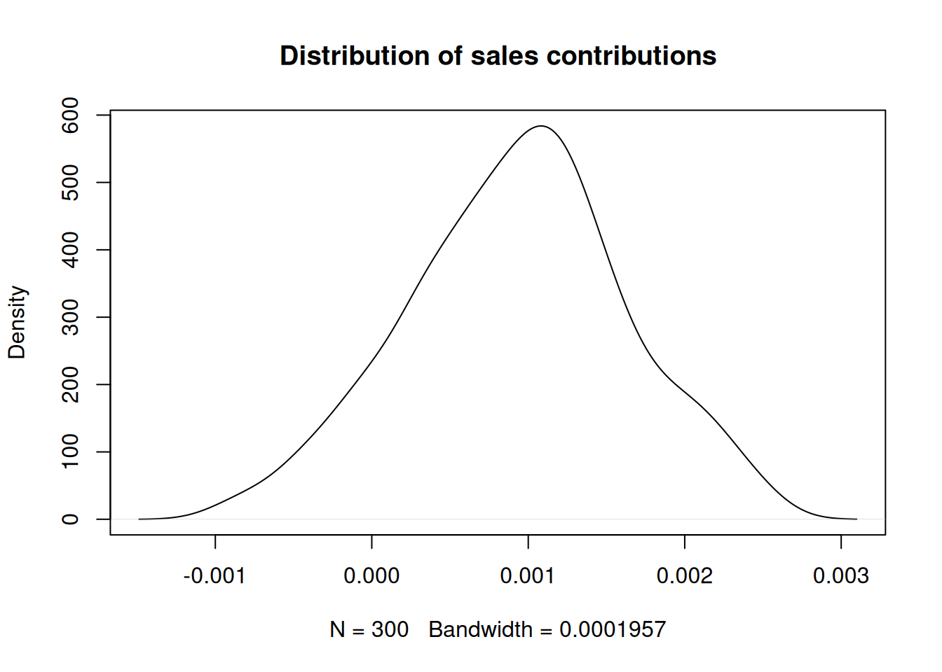
One reason that I’ve not seen for the two-regression approach is that it’s also more convenient to calculate product contributions when doing two regressions.

laspeyres_relatives <- exp(
  predict(mdl2, sales2[[1]]) - predict(mdl1, sales2[[1]])
)
contrib_laspeyres <- gpindex::geometric_contributions(laspeyres_relatives)

paasche_relatives <- exp(
  predict(mdl2, sales2[[2]]) - predict(mdl1, sales2[[2]])
)
contrib_paasche <- gpindex::geometric_contributions(paasche_relatives)

contrib_fisher <- Map(
  `*`,
  gpindex::transmute_weights(0, 1)(c(laspeyres, paasche)),
  list(contrib_laspeyres, contrib_paasche)
)

plot(
  density(unlist(contrib_fisher)),
  main = "Distribution of sales contributions"
)

References

Aizcorbe, Ana M. 2014. A Practical Guide to Price Index and Hedonic Techniques. Oxford University Press. https://doi.org/10.1093/acprof:oso/9780198702429.001.0001.

ILO, IMF, OECD, UNECE, and World Bank. 2013. Handbook on Residential Property Prices Indices (RPPIs). Eurostat. https://doi.org/10.2785/34007.

IMF. 2020. Residential Property Prices Index (RPPI) Practical Compilation Guide. International Monetary Fund. https://www.imf.org/en/Data/Statistics/RPPI-guide.

Wooldridge, Jeffrey M. 2002. Econometric Analysis of Cross Section and Panel Data. MIT Press.

Footnotes

1. This type of regression model comes up in the literature on program evaluation as a way to estimate average treatment effects; see, e.g., Wooldridge (2002, sec. 18.3.1).

2. These standard error are approximate when the mean of the characteristics is calculated from the sample of data used to the fit the model.