How does the difference between the arithmetic and geometric mean depend on variance?

It’s well known that the arithmetic mean is larger than the geometric mean, but how does the difference between these means relate to variance?

That the arithmetic mean of a set of number is larger than the geometric mean is a foundational result in the theory of inequalities. This is a useful result for index numbers in particular as it gives that, for the same data, an index based on an arithmetic mean will always be larger than the corresponding index based on the geometric mean.

The latest edition of the CPI manual says the following about the difference between the arithmetic and geometric mean and how it relates to variance (IMF et al. 2020, 2)

It should be noted that an arithmetic average is always greater than or equal to a geometric average and that the difference will be greater, the greater the variance in the price relatives.

This seems like a great result that gives a way to easily think about the relationship between an index that uses an arithmetic mean to aggregate price relatives (Carli index) and one that uses a geometric mean (Jevons index). Unfortunately it’s not true—see Lord (2002) for a neat way to generate counter examples. ¹

The issue is that, for a vector of positive numbers \(x\in\mathbf{R}_{n}^{++}\), the difference between the arithmetic mean \(\mathfrak{A}(x)\) and geometric mean \(\mathfrak{G}(x)\) is only bounded by the variance (Bullen 2003, 156)

\[ \frac{\text{var}(x)}{2 \max(x)} \leq \mathfrak{A}(x) - \mathfrak{G}(x) \leq \frac{\text{var}(x)}{2 \min(x)}. \]

For two vectors \(x\) and \(y\), we have that \(\mathfrak{A}(y) - \mathfrak{G}(y) > \mathfrak{A}(x) - \mathfrak{G}(x)\) if

\[ \text{var}(y) > \frac{\max(y)}{\min(x)}\text{var}(x) \tag{1}\]

and the opposite if

\[ \text{var}(y) < \frac{\min(y)}{\max(x)}\text{var}(x) \tag{2}\]

If \(\max(y) > \min(x)\) (what we should expect) then the difference between the arithmetic and geometric mean increases with a sufficiently large increase in variance. Similarly, if \(\min(y) < \max(x)\) then the difference between the arithmetic and geometric mean decreases with a sufficiently large decrease in variance. If the support of the distribution is sufficiently narrow then the difference between the arithmetic and geometric mean will follow closely with the variance, and this is similar to the argument that generates the claim in the CPI manual (IMF et al. 2025, 131).

What I want to understand is how the difference between the arithmetic and geometric mean changes for smaller changes in variance without placing restrictions on the support of the distribution. Let’s consider drawing a collection of samples from a fixed probability distribution to see how the difference between the arithmetic and geometric mean relates to variance among samples from that distribution. We’ll make a few helper functions for this.

var_ineq <- function(x) {
  m <- mean(x)
  c(
    var = mean((x - m)^2),
    diff = m - exp(mean(log(x))),
    min = min(x),
    max = max(x)
  )
}

simulate_var_ineq <- function(n, sim, dist) {
  res <- apply(matrix(dist(n * sim), nrow = n), 2, var_ineq)
  res[, order(res["var", ])]
}

prob_decrease <- function(x) {
  apply(
    x,
    2,
    \(z) {
      cond <- x["var", ] <= x["max", ] / z["min"] * z["var"] |
        x["var", ] >= x["min", ] / z["max"] * z["var"]
      x <- x[, cond]
      decrease <- x["diff", ] < z["diff"] & x["var", ] > z["var"]
      increase <- x["diff", ] > z["diff"] & x["var", ] < z["var"]

      mean(decrease | increase) * 100
    }
  )
}

The scatter plot of the difference between the arithmetic and geometric mean and variance for a sample of size 10 shows that, although the difference tends to increase with variance, there are several instances where the opposite occurs.

set.seed(15243)

sim <- simulate_var_ineq(10, 100, \(n) rlnorm(n, sdlog = 0.25))

plot(t(sim), ylab = "arithmetic mean - geometric mean", xlab = "variance")
symbols(0.13, 0.05, circles = 0.015, inches = FALSE, add = TRUE, lty = 2)
symbols(0.065, 0.03, circles = 0.01, inches = FALSE, add = TRUE, lty = 2)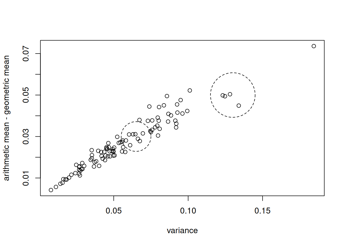

To better understand this, let’s simulate the probability that the difference between the arithmetic and geometric mean decreases with variance, conditional on Equation 1 and Equation 2 not holding.

res <- simulate_var_ineq(10, 5000, \(n) rlnorm(n, sdlog = 0.25)) |>
  prob_decrease()

summary(res)

   Min. 1st Qu.  Median    Mean 3rd Qu.    Max. 
  0.000   4.400   6.340   6.562   8.020  35.160 

Overall, the median of the conditional probability that the difference between the arithmetic and geometric mean decreases with variance is about 6.3%. This is a fairly small probability for the difference between the means to decrease when variance increases, although it depends on the underlying population from which samples are drawn. Drawing samples from a distribution with a wider support makes it more likely to see the the difference between the arithmetic and geometric mean decreases with variance.

res <- simulate_var_ineq(10, 5000, \(n) runif(n, 0.25, 4)) |>
  prob_decrease()

summary(res)

   Min. 1st Qu.  Median    Mean 3rd Qu.    Max. 
  0.020   8.515  13.400  13.579  17.100  50.580 

As the support of the distribution shrinks, the difference between the arithmetic and geometric mean follows the variance more closely and the probabiltity that the difference in means decreases as variance increases becomes small.

res <- simulate_var_ineq(10, 5000, \(n) runif(n, 0.9, 1 / 0.9)) |>
  prob_decrease()

summary(res)

   Min. 1st Qu.  Median    Mean 3rd Qu.    Max. 
  0.000   0.800   1.140   1.194   1.500   4.560 

References

Bullen, P. S. 2003. Handbook of Means and Their Inequalities. Springer Science+Business Media. https://doi.org/10.1007/978-94-017-0399-4.

IMF, ILO, Eurostat, UNECE, OECD, and World Bank. 2020. Consumer Price Index Manual: Concepts and Methods. International Monetary Fund. https://doi.org/10.5089/9781484354841.069 .

———. 2025. Consumer Price Index Manual: Theory. International Monetary Fund. https://doi.org/10.5089/9781513559605.069.

Lord, N. 2002. “Does Smaller Spread Always Mean Larger Product?” The Mathematical Gazette, no. 506, 86: 273–74. https://doi.org/10.2307/3621857.

Footnotes

1. This can also apply to the difference between the arithmetic mean and harmonic mean, where it is often suggested that the difference between these means increases with variance (IMF et al. 2025, 131).